


When you’re operating in information scientific research and analytics, taking care of high-dimensional information belongs of it. You might have a dataset with 600 and even 6000 variables, with some columns that confirm to be essential in modelling, while some that are irrelevant, some associated to every various other (i.e. weight and elevation) and some totally independent of each other.
Due to the fact that taking care of countless functions is both challenging and ineffective, our objective is to lower the dataset to less independent functions that catch the majority of the initial details.
When we lower information from lots of measurements to less measurements, we utilize an analytical method incorporated with information compression. This technique is referred to as Principal Part Evaluation (PCA).
What is Dimensionality Decrease?
Measurement decrease suggests streamlining a dataset by lowering the variety of measurements and concentrating on the essential functions. It can additionally be called an approach that streamlines a high-dimensional dataset right into less measurements by concentrating on the essential functions.
Dimensionality decrease is practical when taking care of datasets which contain a lot of variables. Several of the commonly utilized dimensionality decrease strategies consist of Principal Part Evaluation, Wavelet Changes, Single Worth Disintegration, Linear Discriminant Evaluation, and Generalized Discriminant Evaluation.
What is Principal Part Evaluation?
Principal Part Evaluation is a crucial technique that aids streamline information by lowering its measurements throughout preprocessing. It is an without supervision strategy utilized for lowering the variety of measurements in a dataset.
It takes into consideration the difference within the information factors and does not utilize any kind of details concerning course tags. We lower the information by taking a look at just how much the information factors differ, without utilizing the course tags or reliant variables.
Actions In Principal Part Evaluation with R
These are minority action in primary element evaluation
1. Making the input information constant by systematizing it.
2. Calculation of the covariance matrix for standard dataset worths.
3. Discovering the eigenvalues and eigenvectors of the covariance matrix.
4. Arranging the eigenvalues and eigen vectors .
5. Remove the primary parts from the information and create a brand-new attribute.
6. Map the information onto the primary element axes.
In this write-up, we intend to accomplish 3 major purposes:
1. Comprehending the requirement for measurement decrease
2. Doing PCA and assessing information variant & information structure
3. Figuring out functions that confirm to be most helpful in information discernment
PCA creates primary parts (equivalent to the variety of functions) that are rated in order of difference (PC1 reveals one of the most difference, PC2 the 2nd most, and so forth…).
To comprehend this in even more information, we will certainly service an example dataset utilizing the prcomp() feature in R. I utilized a dataset from data.world, an open system, which reveals the nutrition material of various pizza brand names. To streamline our evaluation, the .csv data consists of just the A, B, and C pizza brand names.
Action 1: Importing collections and reviewing the dataset right into a table
See to it your .csv data remains in the present folder. You can inspect the folder with getwd() or alter it with setwd().
collection(dplyr)
collection(data.table)
collection(datasets)
collection(ggplot2)
information <- data.table(read.csv(“Pizza.csv”))
Step 2: Making sense of the data
These functions tell you a) the dimensions i.e. rows x columns of the matrix b) the first few rows of the data and c) the datatypes of the variables.
dim(data)
head(data)
str(data)
Basic Initial Function
Step 3: Getting the principal components
We want to make our target variable NULL since we want our analysis to tell us the different types of pizza brands there are. Once we have done that and copied our dataset to keep the original values, we’ll runt prcomp() with .scale = TRUE so that the variables are scaled to unit variance before the analysis.
pizzas <- copy(data)
pizzas <- pizza[, brand := NULL]
pca <- prcomp(pizzas, scale. = TRUE)
The important thing to know about prcomp() is that it returns 3 things:
1. x: stores all the principal components of data that we can use to plot graphs and understand the correlations between the PCs.
2. sdev: calculates the standard deviation to know how much variation each PC has in the data
3. rotation: determines which loading scores have the largest effect on the PCA plot i.e., the largest coordinates (in absolute terms)
Download PDF: Principal Component Analysis with R: How to Reduce Dimensionality
Step 4: Using x
Even though currently our data has more than two dimensions, we can plot our graph using x. Usually, the first few PCs capture maximum variance, hence PC1 and PC2 are plotted below to understand the data.
pca_1_2 <- data.frame(pca$x[, 1:2])

plot(pca$x[,1], pca$x[,2])
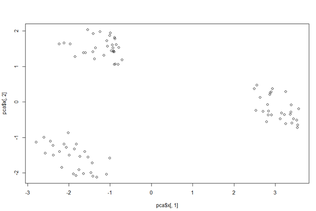
PC1 against PC2 plot
This plot clearly shows us how the first two PCSs divide the data into three clusters (or A, B & C pizza brands) depending on the characteristics that define them.
Step 5: Using sdev
Here, we use the square of sdev and calculate the percentage of variation each PC has.
pca_var <- pca$sdev^2
pca_var_perc <- round(pca_var/sum(pca_var) * 100, 1)
barplot(pca_var_perc, main = "Variation Plot", xlab = "PCs", ylab = "Percentage Variance", ylim = c(0, 100))
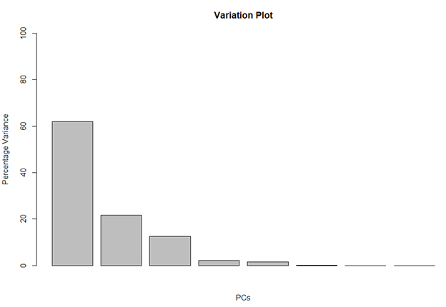
Percentage Variation Plot
This barplot tells us that almost 60% of the variation in the data is shown by PC1, 20% by PC2, 12% by PC3 and then very little is captured by the rest of the PCs.
Step 6: Using rotation
This part explains which of the features matter the most in separating the pizza brands from each other; rotation assigns weights to the features (technically called loadings) and an array of ‘loadings’ for a PC is called an eigenvector.
PC1 <- pca$rotation[,1]
PC1_scores <- abs(PC1)
PC1_scores_ordered <- sort(PC1_scores, decreasing = TRUE)
names(PC1_scores_ordered)
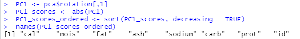
We see how the variable ‘cal’ (Amount of calories per 100 grams in the sample) is the most important feature in differentiating between the brands, while ‘mois’ (Amount of water per 100 grams in the sample) is next and so on.
Step 7: Differentiating between brands using the two most important features
ggplot(data, aes(x=data$cal, y=data$mois, color = data$brand)) + geom_point() + labs(title = "Pizza brands by two variables")
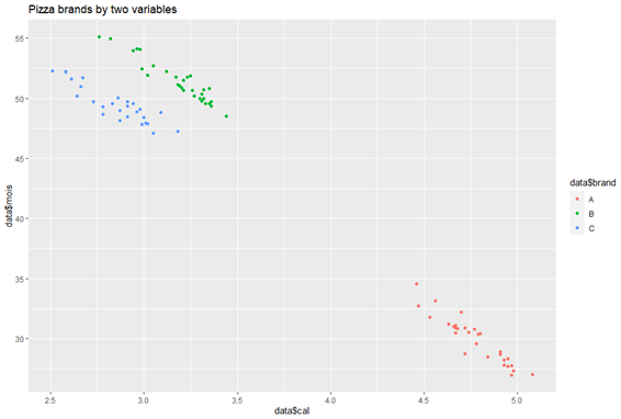
Cluster Formation via Most Weighted Columns
This plot clearly shows how, instead of the 8 columns given to us in the dataset, only two were enough to understand we had three different types of pizzas, thus making PCA a successful analytical tool to reduce high-dimensional data into a lower one for modelling and analytical purposes.
